First printing release date: August 30, 2018. The e-book edition is an electronic, full-page duplicate.
The Kindle edition does not have the back cover. Most of the back cover is a quick index to key topics. Here is a pdf file with that index: Back Cover Index
Errata:
Thanks to Professor Dorota Kuchta for reporting two figure misdirections. Both involve practicing the addition rule formula.
First, on page 157, is a recommendation to practice solving for P(A+B) using the probability tree on page 155. That solution is:
P(A + B) = P(A) + P(B) − P(AB)
= (.12 + .18) + (.12 + .14) − .12
= .30 + .26 − .12 = .44
An easier way is with the complement rule: P(A + B) = 1 − P(not A and not B) = 1 − .56 = .44
Then, also on 157, a few lines down, is a solution for another probability tree:
The numbers are
See if you can confirm the solution: P(A+B) = P(A) + P(B) − P(AB) = 0.902 + 0.855 − 0.812 = 0.945.
Thanks to Yasuf Hamzah for noticing and reporting these problems:
Several equations on pages 25, 53, and 147 may appear corrupted in the Kindle edition, depending upon the Kindle software and/or device. Amazon has been unable to replicate the problem. Contact me if you want PDF copies of these pages as they should appear. Report equations problem
p. 57. The equation near the bottom has a “=” in the middle that should be “+”. The equation should read:
EV Impact = .333($2M) + .667($5M) = $4M.
p. 99 and elsewhere. Utility curve shapes: convex vs. concave. See the discusson in the section, below. Yusuf corrected a miswording the earlier posting.
p. 165. Another "=" that should be a "+". The equation should read
BaseCost = 54 * (1 + CostEscalation)
p. 171. The schematic decision tree (upper figure) has two "New, Fixed" branches. The middle branch label should be "New, Skid".
p. 176. The solutions are transposed. Depending upon the Used Plant inspection outcomes, the best alternative in each is:
o "Favorable" and Used Skid plant
o "UnFavorable" and New Fixed plant
Thanks to Bryn Stevens, PreProject Project Forecasting, South Australia, for his careful reading. Bryn reported several typos and, more importantly, inconsistencies in labeling concave and convex utility functions (see below).
Simple typos:
Chapter 10, p. 154. The 4th line up from the bottom should read, "... probability that \( \overline{\rm {E}} \) occurs."
Chapter 10, p. 160. The 3rd line down from the top should read," P(ABC …) = P(A) × P(B) × P(C) × ..."
Chapter 10, p. 163. There should be a \( \overline{\rm {A}} \) symbol above the table right column.
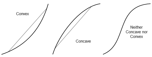
Concave vs. Convex utility functions. I've been inconsistent over my career, and this manifested in the book. Sorry about that. Whether the curve is concave or convex depends upon whether viewing from above or below. Google: "A concave function is also synonymously called concave downwards, concave down, convex upwards, convex cap or upper convex." How confusing is this?!
The next update, the book align with the most-common mathematics function convention, as illustrated and explained on page 98:
General, for any line connecting two points on the function:
If the curve connecting the points is everywhere below the line, the function is convex.
If the curve connecting the points is everywhere above the line, the function is concave.
[Thanks to Yasuf Hamzah for reporting that I had these reversed. ^^ on this page.]
For functions that are twice differentiable and have no straight line segments:
Strictly convex functions have increasing slope everywhere (i.e., the second derivative is positive, and the function is accelerating upward.
Strictly concave functions have decreasing slope everywhere (i.e., the second derivative is negative, and the function is accelerating downward).

Please contact me if you have questions or concerns about anything you read in the book. E-mail: john1@maxvalue.com
Copyright (C) 2018-2022 by John R. Schuyler. Last updated 3-Mar-2022.